Code:
def sphere_tracing(
    self,
    implicit_fn,
    origins, # Nx3
    directions, # Nx3
):
    '''
    Input:
        implicit_fn: a module that computes a SDF at a query point
        origins: N_rays X 3
        directions: N_rays X 3
    Output:
        points: N_rays X 3 points indicating ray-surface intersections. For rays that do not intersect the surface,
                the point can be arbitrary.
        mask: N_rays X 1 (boolean tensor) denoting which of the input rays intersect the surface.
    '''
    # TODO (Q1): Implement sphere tracing
    # 1) Iteratively update points and distance to the closest surface
    #   in order to compute intersection points of rays with the implicit surface
    # 2) Maintain a mask with the same batch dimension as the ray origins,
    #   indicating which points hit the surface, and which do not

    t = torch.ones(origins.shape[0],1).to(get_device()) * self.near    # (N_rays, 1) # Starting query points along each ray
    points = origins + t * directions

    mask = torch.ones_like(t) > 0                 # (N_rays, 1): All True, means intersecting the implicit surface (default)

    eps = 1e-5
    iteration = 0
    while True:
        iteration+=1
        f_p = implicit_fn.get_distance(points)
        t = t + f_p
        points = origins + t * directions
        mask[t > self.far] = False              # Rays that are NOT intersecting the implicit surface
        intersection_point_not_found_yet = f_p[mask] > eps

        if intersection_point_not_found_yet.sum() == 0:
            print("All the rays intersecting the implicit surface have been found!")
            break

        if iteration == self.max_iters:
            print('Maximum iteration reached!')
            break

    return points, mask
Implementation of sphere tracing : iterative method for the ray marching has been used.
pesudo code:
While(f(p)>$\epsilon$):
t <- t + f(p)
p <- origin + t * directions
To compute the mask, it was initialised to be True, that is intercepting with implicit surface. When marching along the ray if the distance exceeds the farthest sample point and yet has not intercepted with the implicit surface we consider the mask to be False.
Code:
class NeuralSurface(torch.nn.Module):
    def __init__(
        self,
        cfg,
    ):
        super().__init__()
        # TODO (Q2): Implement Neural Surface MLP to output per-point SDF
        self.harmonic_embedding_distance = HarmonicEmbedding(3, cfg.n_harmonic_functions_xyz)
        embedding_dim_distance = self.harmonic_embedding_distance.output_dim   # (3*4*2=24)

        self.n_layers_distance = cfg.n_layers_distance # 6
        self.n_hidden_neurons_distance = cfg.n_hidden_neurons_distance #128

        self.in_layer_distance = torch.nn.Linear(embedding_dim_distance, cfg.n_hidden_neurons_distance)
        self.hidden_layer_distance = torch.nn.Linear(cfg.n_hidden_neurons_distance, cfg.n_hidden_neurons_distance)
        self.out_layer_distance = torch.nn.Linear(cfg.n_hidden_neurons_distance, 1)

        self.relu = torch.nn.functional.relu

        # TODO (Q3): Implement Neural Surface MLP to output per-point color
        self.harmonic_embedding_color = HarmonicEmbedding(3, cfg.n_harmonic_functions_xyz)
        embedding_dim_color = self.harmonic_embedding_color.output_dim     # (3*4*2=24)

        self.n_layers_color = cfg.n_layers_color # 2
        self.n_hidden_neurons_color = cfg.n_hidden_neurons_color # 128

        self.in_layer_color = torch.nn.Linear(embedding_dim_color, cfg.n_hidden_neurons_color)
        self.hidden_layer_color = torch.nn.Linear(cfg.n_hidden_neurons_color, cfg.n_hidden_neurons_color) # hidden layer for color
        self.out_layer_color = torch.nn.Linear(cfg.n_hidden_neurons_color, 3) # output layer for color

        self.sigmoid = torch.sigmoid

    def get_distance(
        self,
        points
    ):
        '''
        TODO: Q2
        Output:
            distance: N X 1 Tensor, where N is number of input points
        '''
        points = points.view(-1, 3)

        embedded_distance = self.harmonic_embedding_distance(points)
        x = self.in_layer_distance(embedded_distance)

        for _ in range(self.n_layers_distance):
            x = self.relu(self.hidden_layer_distance(x))

        distance = self.out_layer_distance(x).view(-1,1)           # No ReLU since distances can be negative,

        return distance
MLP description:
Input to the neural network : point clouds sampled on the object.
Output to the neural network : signed distances with respect to the object.
Thus, the groundtruth of the output should just be zeros, representing the surface (roots of an implicit function is zero at the surface of the object). Six fully connected hidden layers with 128 hidden units each have been used. ReLu activation has been used for every layer. The last layer comprised of a single neuron without any activation as the output distances can range in any value in the real number line.
def eikonal_loss(gradients):
    # TODO (Q2): Implement eikonal loss on Nx3 gradients
    gradients_norm = torch.norm(gradients, dim=-1)
    return torch.abs(gradients_norm - torch.ones_like(gradients_norm)).mean()
Eikonal loss was to enforce the gradient of SDF respect to x to have norm of 1 as a regulation term.
$$ L_{reg} = \frac{1}{N}\sum(||\nabla_{x_i} f(x_i;\theta)||_2-1)\ $$ where, $x_i \in X$ represents the point in the pointcloud ; $\theta$ represent the learning parameters.
This loss encourages the coordinate-based network to predict the closest offset to surface instead of arbitary values for points in space.
Point cloud used for training:
 Prediction of surface:

Color Prediction code:
class NeuralSurface(torch.nn.Module):
    def __init__(
        self,
        cfg,
    ):
        super().__init__()
        # TODO (Q2): Implement Neural Surface MLP to output per-point SDF
        self.harmonic_embedding_distance = HarmonicEmbedding(3, cfg.n_harmonic_functions_xyz)
        embedding_dim_distance = self.harmonic_embedding_distance.output_dim   # (3*4*2=24)

        self.n_layers_distance = cfg.n_layers_distance # 6
        self.n_hidden_neurons_distance = cfg.n_hidden_neurons_distance #128

        self.in_layer_distance = torch.nn.Linear(embedding_dim_distance, cfg.n_hidden_neurons_distance)
        self.hidden_layer_distance = torch.nn.Linear(cfg.n_hidden_neurons_distance, cfg.n_hidden_neurons_distance)
        self.out_layer_distance = torch.nn.Linear(cfg.n_hidden_neurons_distance, 1)

        self.relu = torch.nn.functional.relu

        # TODO (Q3): Implement Neural Surface MLP to output per-point color
        self.harmonic_embedding_color = HarmonicEmbedding(3, cfg.n_harmonic_functions_xyz)
        embedding_dim_color = self.harmonic_embedding_color.output_dim     # (3*4*2=24)

        self.n_layers_color = cfg.n_layers_color # 2
        self.n_hidden_neurons_color = cfg.n_hidden_neurons_color # 128

        self.in_layer_color = torch.nn.Linear(embedding_dim_color, cfg.n_hidden_neurons_color)
        self.hidden_layer_color = torch.nn.Linear(cfg.n_hidden_neurons_color, cfg.n_hidden_neurons_color) # hidden layer for color
        self.out_layer_color = torch.nn.Linear(cfg.n_hidden_neurons_color, 3) # output layer for color

        self.sigmoid = torch.sigmoid

    def get_distance(
        self,
        points
    ):
        '''
        TODO: Q2
        Output:
            distance: N X 1 Tensor, where N is number of input points
        '''
        points = points.view(-1, 3)

        embedded_distance = self.harmonic_embedding_distance(points)
        x = self.in_layer_distance(embedded_distance)

        for _ in range(self.n_layers_distance):
            x = self.relu(self.hidden_layer_distance(x))

        distance = self.out_layer_distance(x).view(-1,1)           # No ReLU since distances can be negative,

        return distance


    def get_color(
        self,
        points
    ):
        '''
        TODO: Q3
        Output:
            distance: N X 3 Tensor, where N is number of input points
        '''
        points = points.view(-1, 3)

        embedded_color = self.harmonic_embedding_color(points)
        x = self.in_layer_color(embedded_color)

        for _ in range(self.n_layers_color):
            x = self.relu(self.hidden_layer_color(x))

        color = self.sigmoid(self.out_layer_color(x)).view(-1,3)
        return color


    def get_distance_color(
        self,
        points
    ):
        '''
        TODO: Q3
        Output:
            distance, points: N X 1, N X 3 Tensors, where N is number of input points
        You may just implement this by independent calls to get_distance, get_color
            but, depending on your MLP implementation, it maybe more efficient to share some computation
        '''

        distances = self.get_distance(points)
        colors = self.get_color(points)
        return distances, colors


    def forward(self, points):
        return self.get_distance(points)

    def get_distance_and_gradient(
        self,
        points
    ):
        has_grad = torch.is_grad_enabled()
        points = points.view(-1, 3)

        # Calculate gradient with respect to points
        with torch.enable_grad():
            points = points.requires_grad_(True)
            distance = self.get_distance(points)
            gradient = autograd.grad(
                distance,
                points,
                torch.ones_like(distance, device=points.device),
                create_graph=has_grad,
                retain_graph=has_grad,
                only_inputs=True
            )[0]

        return distance, gradient
SDF to Density code:
def sdf_to_density(signed_distance, alpha, beta):
    # TODO (Q3): Convert signed distance to density with alpha, beta parameters
    s = - signed_distance

    PSI_beta = torch.zeros_like(signed_distance)
    PSI_beta[s<=0] = (0.5 * torch.exp(s / beta))[s<=0]
    PSI_beta[s>0] = (1 - 0.5 * torch.exp( - s / beta))[s>0]
    density = alpha * PSI_beta

    return density
Intuitive explanation of what the parameters alpha and beta are doing:
alpha controls the overall density. It is a scaling term in front of the function;
beta controls the smoothing amount, meaning how much is the density sensitive to distance changes. If beta approaches to zero, the density close to the surface would be changing dramatically.
How does high beta bias your learned SDF? What about low beta?
High beta causes the density to be less sensitive near surface and the rendering would be more blurred. On the contrary, low beta results density highly sensitive near surface such that the surface is more accurately rendered.
Would an SDF be easier to train with volume rendering and low beta or high beta? Why?
Right values of beta would make SDF easier to train.
High beta would make training and volume rendering more stable, as sharp transition from empty to occupied space would be mitigated. However, the exact surface would be well-extracted and optimized.
On the other hand, low beta results too small margin for surface have nonzero density, so the volume rendering and training may be harder.
So there's some good value of beta lying in between.
Would you be more likely to learn an accurate surface with high beta or low beta? Why?
To learn an accurate surface it is more likely achieved with a low beta value. This is because the density function in this case converges to a indicator function: as density close to surface would be $0.5\alpha$ and zeros elsewhere.
RESULTS:
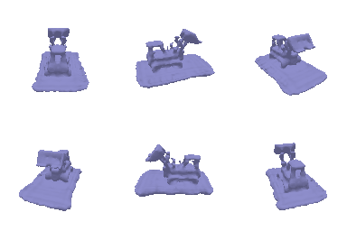
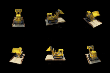
At the end of 230 epochs: Setting $lr= 0.001$, $chunk\_size= 8192$ and keeping the rest of hyperparameters as given:
SDF -> volume density:
 Per-point color prediction:

|

|

|
|

|

|
No Mesh generated

|

|
|
Surface Normal Recovery code:
def get_surface_normal(
    self,
    points
):
    '''
    TODO: Q4
    Input:
        points: N X 3 Tensor, where N is number of input points
    Output:
        surface_normal: N X 3 Tensor, where N is number of input points
    '''

    #  This can be done by dividing the gradient by its norm
    _, gradients = self.get_distance_and_gradient(points=points)            # torch.Size([524288, 3])
    gradients_norm = torch.norm(gradients, dim=-1, keepdim=True)              # torch.Size([524288])
    return torch.divide(gradients,gradients_norm)
Phong Reflection Model code:
def phong(
    normals,
    view_dirs,
    light_dir,
    params,
    colors
):
    # TODO: Implement a simplified version Phong shading
    # Inputs:
    #   normals: (N x d, 3) tensor of surface normals
    #   view_dirs: (N x d, 3) tensor of view directions
    #   light_dir: (3,) tensor of light direction
    #   params: dict of Phong parameters
    #   colors: (N x d, 3) tensor of colors
    # Outputs:
    #   illumination: (N x d, 3) tensor of shaded colors
    #
    # Note: You can use torch.clamp to clamp the dot products to [0, 1]
    # Assume the ambient light (i_a) is of unit intensity
    # While the general Phong model allows rerendering with multiple lights,
    # here we only implement a single directional light source of unit intensity
    # pass
    ka, ks, kd, alpha = params["ka"], params["ks"], params["kd"], params["n"]

    Ia = torch.ones_like(colors).to(get_device())    # (N x d, 3)
    # Ia = torch.nn.functional.normalize(torch.ones_like(colors), dim=-1).to(get_device())    # (N x d, 3)
    # Ia = torch.nn.functional.normalize(colors, dim=-1).to(get_device())
    light_dir = torch.nn.functional.normalize(light_dir)                   # (3,)
    normals = torch.nn.functional.normalize(normals)                       # (N x d, 3)

    R = (2 * torch.sum(light_dir * normals, dim=-1, keepdim=True)) * normals - light_dir                    # (N x d, 3)
    R = torch.nn.functional.normalize(R, dim=-1)                           # (N x d, 3)

    view_dirs = torch.nn.functional.normalize(view_dirs)                   # (N x d, 3)

    # a = ka * Ia
    a = ka
    d = kd * torch.clamp(torch.sum(light_dir * normals, dim=-1, keepdim=True), 0, 1)
    s = ks * (torch.clamp(torch.sum(R * view_dirs, dim=-1, keepdim=True), 0, 1) ** alpha)

    illumination = torch.clamp(a + d + s,0.,1.)*colors   # torch.zeros_like(colors)

    return illumination
light_dir = light_location - origin #None #TODO: Use light location and origin to compute light direction
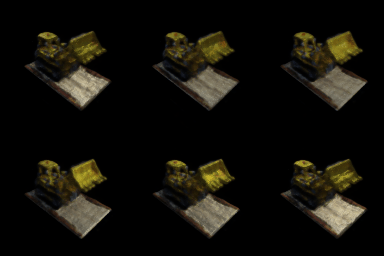
Model under rotating lights:

|
|
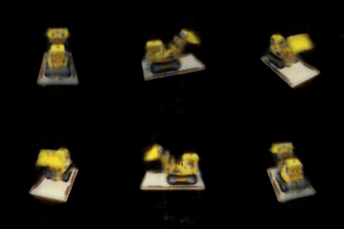
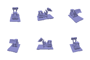
Randomly 20 images from train_idx were chosen for training. VolSDF was easily trainable and showed decent results:
|

|
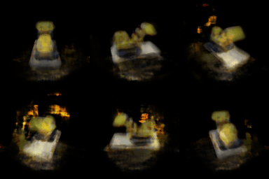
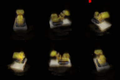
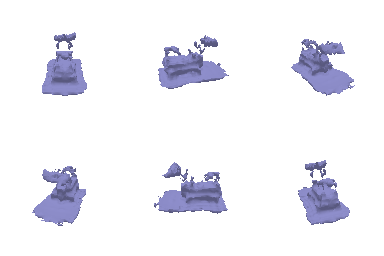
On the contrary using same set of training samples, Nerf was not able to converge and resulted in empty output:

|
We can conclude that VolSDF needs less training views than Nerf.
This is because for VolSDF we need to train the implicit SDF, and then the density is analytically calculated afterwards, unlike in Nerf which is learns the volumetric representations. The information that needed to learn for VolSdf is much less as compared to that of Nerf.
Used the 'naive' solution from the NeuS paper: $$ \phi_s(x) = \frac{se^{-sx}}{(1+e^{-sx})} $$
def sdf_to_density_naive(signed_distance, scale):
    density = scale * torch.exp(-scale * signed_distance) / torch.square(1.0 + torch.exp(-scale* signed_distance))
    return density
Results for different scale parameter, $s$:

|

|

|
|

|

|
|

|