16-825 Assignment 2: Single View to 3D

Late days: 2

Sayan Mondal

Goals: In this assignment, you will explore the types of loss and decoder functions for regressing to voxels, point clouds, and mesh representation from single view RGB input.

1. Exploring loss functions

1.1. Fitting a voxel grid (5 points)

Optimized voxel grid:

Ground truth voxel grid:

1.2. Fitting a point cloud (5 points)

Optimized point cloud:

Ground truth point cloud:

1.3. Fitting a mesh (5 points)

Optimized mesh:

Ground truth mesh:

2. Reconstructing 3D from single view

2.1. Image to voxel grid (20 points)

Docoder Model:

self.decoder = nn.Sequential(
                nn.Linear(512,512),
                nn.ReLU(True),
                nn.Unflatten(1, torch.Size([1, 8, 8, 8])),
                # torch.Size([10, 512]) -> torch.Size([b, 1, 8, 8, 8])

                nn.ConvTranspose3d(in_channels=1, out_channels=4, kernel_size=3, stride=1),
                nn.ReLU(True),   
                # torch.Size([b, 1, 8, 8, 8]) -> torch.Size([b, 4, 10, 10, 10])

                nn.ConvTranspose3d(in_channels=4, out_channels=8, kernel_size=3, stride=1),
                nn.ReLU(True),
                # torch.Size([b, 4, 10, 10, 10]) -> torch.Size([b, 8, 12, 12, 12])

                nn.ConvTranspose3d(in_channels=8, out_channels=16, kernel_size=5, stride=1),
                nn.ReLU(True),
                # torch.Size([b, 8, 12, 12, 12]) -> torch.Size([b, 16, 16, 16, 16])
    
                nn.ConvTranspose3d(in_channels=16, out_channels=8, kernel_size=7, stride=1),
                nn.ReLU(True),
                # torch.Size([b, 16, 16, 16, 16]) -> torch.Size([b, 8, 22, 22, 22])

                nn.ConvTranspose3d(in_channels=8, out_channels=4, kernel_size=9, stride=1),
                nn.ReLU(True),
                # torch.Size([b, 8, 22, 22, 22]) -> torch.Size([b, 4, 30, 30, 30])

                nn.ConvTranspose3d(in_channels=4, out_channels=1, kernel_size=3, stride=1)
                # torch.Size([b, 4, 30, 30, 30]) -> torch.Size([b, 1, 32, 32, 32])
            )

Run:

python train_model.py --type 'vox' --batch_size 64 --num_workers 4 --save_freq 100

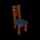
Example 1 in the test set:

Input RGB:

Render of the predicted 3D voxel grid :

Render of the ground truth mesh:

Example 2 in the test set:

Input RGB:

Render of the predicted 3D voxel grid :

Render of the ground truth mesh:

Example 3 in the test set:

Input RGB:

Render of the predicted 3D voxel grid :

Render of the ground truth mesh:

2.2. Image to point cloud (20 points)

Decoder Model:

self.decoder =  nn.Sequential(
                nn.Linear(512, 512),
                nn.ReLU(True),
                nn.Unflatten(dim=1, unflattened_size= (512, 1)),
                # torch.Size([b, 512])  ->  torch.Size([b, 512, 1])

                nn.Conv1d(in_channels= 512, out_channels= 1024, kernel_size=1),
                nn.BatchNorm1d(num_features=1024),
                nn.ReLU(True),
                # torch.Size([b, 512, 1]) ->  torch.Size([b, 1024, 1])

                nn.Conv1d(in_channels= 1024, out_channels= 2048, kernel_size=1),
                nn.BatchNorm1d(num_features=2048),
                nn.ReLU(True),
                # torch.Size([b, 1024, 1]) ->  torch.Size([b, 2048, 1]) 

                nn.Conv1d(in_channels= 2048, out_channels= self.n_point*3, kernel_size=1),
                # torch.Size([b, 2048, 1]) ->  torch.Size([b, self.n_point*3, 1])

            )

Run:

python train_model.py --type 'point' --batch_size 64 --num_workers 4 --save_freq 100 --lr 1e-3

Example 1 in the test set:

Input RGB:

Render of the predicted 3D point cloud:

Render of the ground truth mesh:

Example 2 in the test set:

Input RGB:

Render of the predicted 3D point cloud:

Render of the ground truth mesh:

Example 3 in the test set:

Input RGB:

Render of the predicted 3D point cloud:

Render of the ground truth mesh:

2.3. Image to mesh (20 points)

Decoder Model:

self.decoder =  nn.Sequential(
                nn.Linear(in_features=512, out_features=1024),
                nn.ReLU(True),
                # torch.Size([b, 512]) ->  torch.Size([b, 1024])

                nn.Linear(in_features=1024, out_features= 2048),
                nn.ReLU(True),
                 # torch.Size([b, 1024]) ->  torch.Size([b, 2048])

                nn.Linear(in_features=2048, out_features= 4096),
                nn.ReLU(True),
                 # torch.Size([b, 2048]) ->  torch.Size([b, 4096])

                nn.Linear(in_features=4096, out_features= mesh_pred.verts_packed().shape[0] * 3),
                 # torch.Size([b, 4096]) ->  torch.Size([b, mesh_pred.verts_packed().shape[0] * 3])
            )

Run:

python train_model.py --type 'mesh' --batch_size 32 --num_workers 4 --save_freq 50 --w_smooth 0.2

Example 1 in the test set:

Input RGB:

Render of the predicted mesh:

Render of the ground truth mesh:

Example 2 in the test set:

Input RGB:

Render of the predicted mesh:

Render of the ground truth mesh:

Example 3 in the test set:

Input RGB:

Render of the predicted mesh:

Render of the ground truth mesh:

2.4. Quantitative comparisions(10 points)

Avg F1 @ 0.05: 87.042 - voxel
Avg F1 @ 0.05: 93.437 - point
Avg F1 @ 0.05: 95.536 - mesh

We find that F-score of mesh >= point cloud > voxel. There can be two possible reasons for this:

• Why voxel< pc and mesh : We used chamfer loss to optimize point cloud and mesh but binary cross entropy loss for voxel, and F1 score is measuring the closeness of predicted points and ground truth.It may not be a friendly indicator for voxels; Also, because of the sampling method for voxel and it is too small (32x32x32), it may not be accurate enough.
• Why mesh > pc : Although not too much difference, in my case mesh get higher score because mesh was trained using higher smootheness loss weight, higher weight of smooth loss typically increases F-score

f1-score curve at different thresholds for voxelgrid:

f1-score curve at different thresholds for pointcloud:

f1-score curve at different thresholds for mesh:

2.5. Analyse effects of hyperparms variations (10 points)

I analyzed the effect of w_chamfer (weight of chamfer loss) for mesh.

Run:

python train_model.py --type 'mesh' --batch_size 32 --num_workers 4 --save_freq 50 --w_chamfer 0.1|3.0|50 --max_iter 2500

For consistancy each model was trained with 2500 iterations and using same hyperparameters, except w_chamfer.

Keeping w_smooth as 0.1, when I increase the w_chamfer from 0.1 to 3, it seems that the predicted output mesh gets less spiky (becomes more smoother). But on increasing w_chamfer to 50, make the prediction more spiky, maybe because the loss has now been increased by a lot and 2500 iterations was not sufficient for the model to converge. Suprisingly, the F1-score for all three cases is quite high (around 92).

Test RGB image:

Test render of the groundtruth mesh:

w_chamfer=0.1---> render of the predicted mesh:

w_chamfer=3.0---> render of the predicted mesh:

w_chamfer=50---> render of the predicted mesh:

w_chamfer = 0.1 ---> f1-score curve at different thresholds for mesh:

w_chamfer = 3.0 ---> f1-score curve at different thresholds for mesh:

w_chamfer = 50 ---> f1-score curve at different thresholds for mesh:

Clearly, F1 score @ 0.05, for all three cases are almost the same (close to 92).

2.6. Interpret your model (15 points)

A visual feature that has been added is to visualize the likelihood of our predicted voxel, so that we can see distribution of the probability and improve our model. To implement this, voxels that are in same range of likelihood are grouped togther, and then textures of different colors accordingly are incorporated and finally they have been rendered together. Color from red to blue as indicator of likelihood from high to low.

Visualizations of my previous trained model for a test case is shown below:

Input RGB:

Render of the groudtruth mesh:

Likelihood voxel representation: